Tutorial 2 - Fish Habitat Assessment using the MesoHABSIM Model
This tutorial demonstrates how to use the SARAwater package to assess fish habitat using the MesoHABSIM model.
Import libraries
[1]:
import os
import pandas as pd
import numpy as np
import matplotlib.pyplot as plt
import sarawater as sara

plt.style.use("stylesheet.mplstyle")
I/O paths and directories creation
[2]:
input_csv_filepath = os.path.join("data", "daily_discharge_30y.csv")
Read the discharge data and create a reach object
Read the CSV data
[ ]:
reach_df = pd.read_csv(input_csv_filepath)

# Convert the first column to datetime
reach_df["Date"] = pd.to_datetime(reach_df["Date"])

# Convert the datetime column to a list of datetime objects
datetime_list = [t.to_pydatetime() for t in reach_df["Date"].tolist()]

# Put the discharge data into a numpy array
discharge_data = np.array(reach_df["Q"].to_list())
Initialize a reach object
[4]:
Qabs_max = 0.2
my_reach = sara.Reach("My Reach", datetime_list, discharge_data, Qabs_max)
Add scenarios to the reach object
Minimum release scenario (read from CSV)
[5]:
# Read the minimum release values from CSV relative to a Minimum Flow Requirement (MFR) policy
minrel_df = pd.read_csv(
    os.path.join("data", "minimum_flow_requirements.csv"), header=None
)

# Get the minimum release values (second column), convert l/s to m3/s
Qreq_months = np.array(minrel_df[1].tolist()) / 1000.0

# Create a constant scenario with these values
MFR_scenario = sara.ConstScenario(
    name="MFR",
    description="Minimum Flow Requirement scenario from CSV file",
    reach=my_reach,
    Qreq_months=Qreq_months,
)

# Add the scenario to the reach
my_reach.add_scenario(MFR_scenario)

# Print the min and max MFR values
min_mfr = MFR_scenario.Qreq_months.min()
max_mfr = MFR_scenario.Qreq_months.max()
print(f"MFR values range from {min_mfr:.3f} to {max_mfr:.3f} [m^3/s]")
MFR values range from 0.090 to 0.106 [m^3/s]
Ecological scenario (using the built-in method)
[6]:
my_reach.add_ecological_flow_scenario(
    "EF", "Ecological Flow Scenario with default parameters"
)
[6]:
Scenario(name=EF, description=Ecological Flow Scenario with default parameters, reach=My Reach)
Let’s check we added the scenarios correctly
[7]:
my_reach.print_scenarios()
scenarios[0]: MFR | Minimum Flow Requirement scenario from CSV file
scenarios[1]: EF | Ecological Flow Scenario with default parameters
Compute the released flow discharge and abstracted flow for each scenario
[8]:
for scenario in my_reach.scenarios:
    scenario.compute_Qrel()
    scenario.compute_natural_abstracted_volumes()
Habitat analysis
Read Habitat-Discharge curves from input data
[ ]:
HQ_curve_df = pd.read_csv(
    os.path.join("data", "HQ_curves.txt"), sep="\t", header="infer"
)
my_reach.add_HQ_curve(HQ_curve_df)
[ ]:
my_reach.get_list_available_HQ_curves()
Compute IH for each species and scenario
[ ]:
for scenario in my_reach.scenarios:
    scenario.compute_IH_for_species()
    for species in scenario.IH.keys():
        print(
            f"Scenario {scenario.name}, Species {species}, IH: {scenario.IH[species]['IH']}"
        )
Draw Plots
Initialize a ReachPlotter object
[12]:
plotter = sara.ReachPlotter(my_reach)
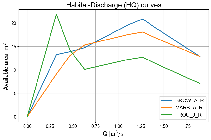
Full HQ curves
[13]:
plotter.plot_hq_curves()
[13]:
<Axes: title={'center': 'Habitat-Discharge (HQ) curves'}, xlabel='Q $[\\mathrm{m}^3/\\mathrm{s}]$', ylabel='Available area $[\\mathrm{m}^2]$'>
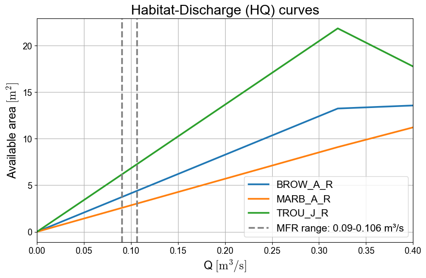
HQ curves setting xlim, and showing the DMV (or another constant scenario) range
[14]:
plotter.plot_hq_curves(xlim=0.4, rule_min=min_mfr, rule_max=max_mfr, rule_name="MFR")
[14]:
<Axes: title={'center': 'Habitat-Discharge (HQ) curves'}, xlabel='Q $[\\mathrm{m}^3/\\mathrm{s}]$', ylabel='Available area $[\\mathrm{m}^2]$'>
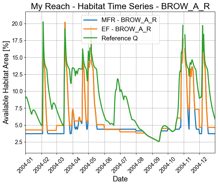
Habitat timeseries
[15]:
my_reach.get_list_available_HQ_curves()
[15]:
['BROW_A_R', 'MARB_A_R', 'TROU_J_R']
[16]:
plotter.plot_habitat_timeseries("BROW_A_R", start_year=2004, end_year=2004, save=True)
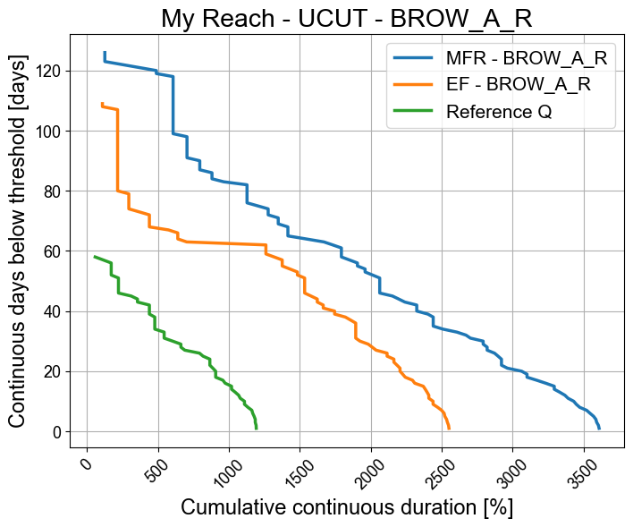
UCUT
[17]:
plotter.plot_ucut_curves("BROW_A_R")
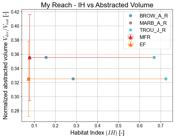
IH_vs_volume
[18]:
plotter.plot_ih_vs_volume(save=True)
[18]:
<Axes: title={'center': 'My Reach - IH vs Abstracted Volume'}, xlabel='Habitat Index $(IH)$ [-]', ylabel='Normalized abstracted volume $V_{der}/V_{nat}$ [-]'>